Using Autofilter in VBA (Part 2)

In the article using Autofilter in VBA (Part 1) Emergenceingames.com introduced you to Autofilter, how Autofilter formula, … . In the article Using Autofilter in VBA (Part 2) below, Emergenceingames.com will introduce you to some examples to visualize how to use Autofilter in VBA.

The following article Emergenceingames.com will introduce you to some examples of how to use Autofilter in VBA. In addition, readers can refer to some existing articles on Emergenceingames.com to learn more about the TRIM function, the DIR function in VBA.

1. Example of Autofilter in VBA

Here are some examples of how to use Autofilter in VBA:

1.1 Example 1: Filter data based on Text . condition

Suppose you have a data file like below and want to filter the data based on the Item column:

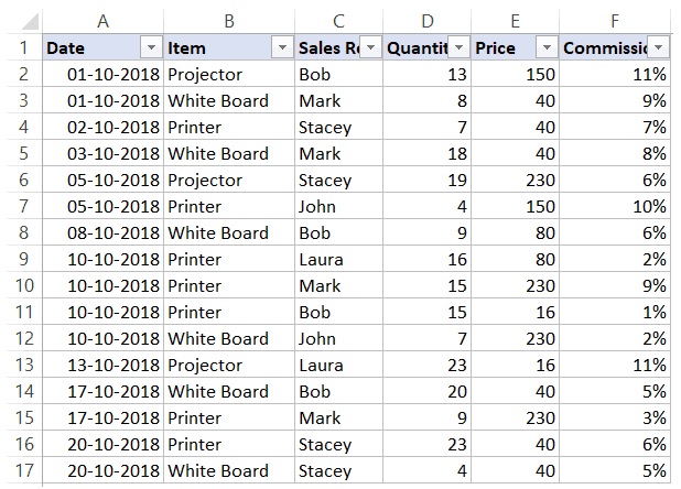
The below code will filter all rows, where the entries are Printer:

Sub FilterRows()

Worksheets(“Sheet1”).Range(“A1″).AutoFilter Field:=2, Criteria1:=”Printer”

End Sub

The above code refers to worksheet 1 and in the worksheet it refers to cell A1 (which is the cell in the data set).

Notice in this example we use Field:=2because the Item column is the 2nd column in the dataset, counting from the left.

1.2 Example 2: Filter data by multiple criteria (AND / OR) in the same column

Let’s say we have the same dataset and want to filter all records where the entries are Printer or Projector:

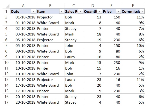
To do this, we will use the following code:

Sub FilterRowsOR()

Worksheets(“Sheet1”).Range(“A1″).AutoFilter Field:=2, Criteria1:=”Printer”, Operator:=xlOr, Criteria2:=”Projector”

End Sub

Note, in the above code we use the xlOR operator. This tells VBA to use both criteria and filter the data if any of the two criteria is met.

Similarly, we can also use AND criteria.

For example, if we want to filter all records whose count is greater than 10 but less than 20, we can use the following code:

Sub FilterRowsAND()

Worksheets(“Sheet1”).Range(“A1″).AutoFilter Field:=4, Criteria1:=”>10”, _

Operator:=xlAnd, Criteria2:=”

End Sub

1.3 Example 3: Filter data by multiple criteria but different columns

Suppose we have the following data file:

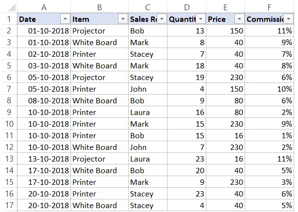
With Autofilter, we can filter multiple columns at once.

For example, if we want to filter all records where the Printer and Sales Rep entries are Mark, we can use the following code:

Sub FilterRows()

With Worksheets(“Sheet1”).Range(“A1”)

.AutoFilter field:=2, Criteria1:=”Printer”

.AutoFilter field:=3, Criteria1:=”Mark”

End With

End Sub

1.4 Example 4: Using Autofilter to filter Top 10 . data

Suppose we have the following data table:

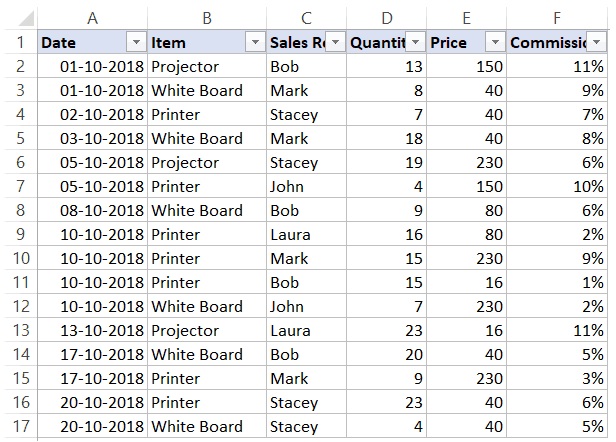
Use the below code to filter the top 10 records (based on the Quantity column):

Sub FilterRowsTop10()

ActiveSheet.Range(“A1″).AutoFilter Field:=4, Criteria1:=”10”, Operator:=xlTop10Items

End Sub

In the example above, the worksheet is named ActiveSheet. You can replace it with your spreadsheet name.

Note, in the above example if we want the top 5 items, we just need to change the number in Criteria1:=”10” from 10 to 5.

The code used to get the top 5 items has the form:

Sub FilterRowsTop5()

ActiveSheet.Range(“A1″).AutoFilter Field:=4, Criteria1:=”5”, Operator:=xlTop10Items

End Sub

No matter how many top items we want to get, the operator value is always xlTop10Items.

Similarly, to get the top 10 lowest entries, we use the following code:

Sub FilterRowsBottom10()

ActiveSheet.Range(“A1″).AutoFilter Field:=4, Criteria1:=”10”, Operator:=xlBottom10Items

End Sub

1.5 Example 5: Filter 10% of data using AutoFilter . method

We continue to use the data table in the above example.

Use the below code to get the top 10% of records (based on the Quantity column):

Sub FilterRowsTop10()

ActiveSheet.Range(“A1″).AutoFilter Field:=4, Criteria1:=”10”, Operator:=xlTop10Percent

End Sub

Since there are 20 records in our data table, the above code will return the top 2 records (10% of total records).

1.6 Example 6: Using wildcards in Autofilter

Given the data table as below:

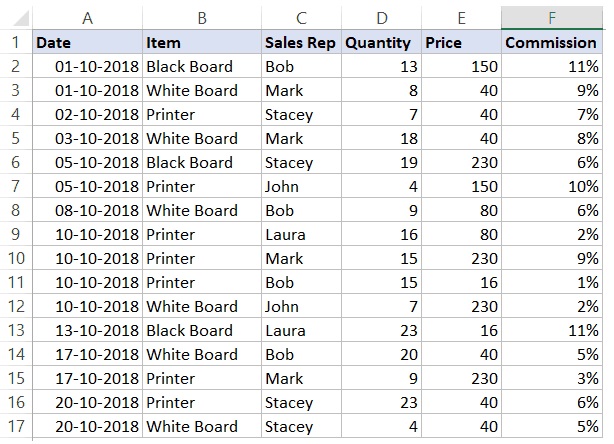
To filter all rows with the name of items containing the word Board, we use the below code:

Sub FilterRowsWildcard()

Worksheets(“Sheet1”).Range(“A1″).AutoFilter Field:=2, Criteria1:=”*Board*”

End Sub

In the above code, we use wildcard * (asterisk) before and after the word Board (which is the criterion).

An asterisk can represent any number of characters. So the above code will filter any entries that have the word Board in them.

1.7 Example 7: Copy filtered rows to new worksheet

If we want to filter the records based on the criteria and copy the filtered rows, we can use the following macro. The macro will copy the filtered rows, add a new worksheet, then paste the filtered rows into the new worksheet:

Sub CopyFilteredRows()

Dim rng As Range

Dim ws As Worksheet

If Worksheets(“Sheet1”).AutoFilterMode = False Then

MsgBox “nothing can be found”

Exit Sub

EndIf

Set rng = Worksheets(“Sheet1”).AutoFilter.Range

Set ws = Worksheets.Add

rng.Copy Range(“A1”)

End Sub

The above code will check if there are filtered rows in Sheet1 or not. If no rows are filtered, it displays a message dialog.

If there are filtered rows, it copies those rows, inserts a new worksheet, and pastes the filtered rows into the newly inserted worksheet.

1.8 Example 8: Copy filtered columns to a new worksheet

If we want to filter the records based on the criteria and copy the filtered columns, we can use the following macro. The macro will copy the filtered columns, add a new worksheet, and then paste these columns into the new worksheet:

Sub CopyFilteredRows()

Dim rng As Range

Dim ws As Worksheet

If Worksheets(“Sheet1”).AutoFilterMode = False Then

MsgBox “nothing can be found”

Exit Sub

EndIf

Set rng = Worksheets(“Sheet1”).AutoFilter.Range

Set ws = Worksheets.Add

rng.Copy Range(“A1”)

End Sub

The above code will check if there are filtered columns in Sheet1 or not. If no columns are filtered, it will display a message dialog.

If there are filtered columns, it copies those columns, inserts a new worksheet, and pastes the filtered columns into the newly inserted worksheet.

1.9 Example 9: Filter data based on cell value

By using Autofilter in VBA with drop down menu we can create a function where when selecting an item in the menu all records of that item will be filtered.

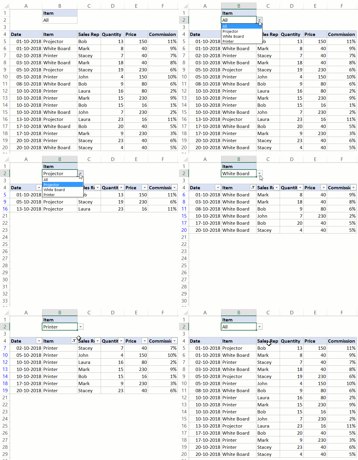
This type of structure can be useful in cases where you want to filter data quickly and then use it for other tasks.

To do this, we use the following code:

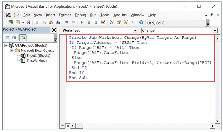
Private Sub Worksheet_Change(ByVal Target As Range)

If Target.Address = “$B$2” Then

If Range(“B2”) = “All” Then

Range(“A5”).AutoFilter

Else

Range(“A5”).AutoFilter Field:=2, Criteria1:=Range(“B2”)

EndIf

EndIf

End Sub

It is the spreadsheet event code, which is only executed when there is a change in the worksheet and the target cell is B2 (where we have the dropdown).

Also if If Then Else condition is used to check if user selected All from the menu or not. If All selected, all data will be displayed.

Note this code is not placed in module. Instead we put in the backend of the spreadsheet with this data.

Follow the steps below to place the code in the spreadsheet code window:

Step 1: Open the VB Editor (by using the keyboard shortcut Alt + F11).

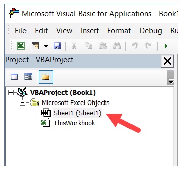
Step 2: In the Project Explorer panel, double-click the worksheet name to which you want to apply this filter.

Step 3: On the spreadsheet code window, copy and paste the code above.

Step 4: Close the VB Editor window.

From now on when using the drop-down menu, it will automatically filter the data.

https://thuthuat.Emergenceingames.com/su-dung-autofilter-trong-vba-phan-2-45661n.aspx
The article Using Autofilter in VBA (Part 2) above Emergenceingames.com has just introduced you to some examples of how to use Autofilter in VBA. If you have any questions or concerns, you can leave your comments in the comment section below the article.